Grocery
Data Analysis.

Grocery Data Analysis in SQL with Python Preprocessing

Executive Summary

The analysis of the store's sales data has revealed valuable insights into product popularity, customer spending behaviors, and geographic purchasing patterns. 'Yogurt Tubes' have been identified as the top-selling product, suggesting a key area for driving sales and promotional strategies. Customer segmentation has effectively categorized individuals into 'High Spenders' and 'Frequent Buyers', which can be targeted with personalized marketing and loyalty programs. Cities like Tucson, Fort Wayne, and Columbus showed high purchase frequencies, pointing towards the potential for targeted regional strategies. The data analysis also highlighted the need for data quality improvements, as significant corrections were required in Python before the data could be loaded into a SQL database. Issues ranged from incorrect delimiters and encoding in CSV files to formatting errors in date-time and price data, suggesting a need for better data management practices.

Part 1 – Questions for Analysis

This analysis of grocery sales data focuses on three areas – Sales Insights, Product Performance, and Customer Analysis. They each offer valuable perspectives on the business. Here's a breakdown of each and the potential value they could provide:

1. Sales Insights:

Importance: Sales data is a direct reflection of business performance. By analyzing sales, you can understand revenue trends, the effectiveness of marketing and sales strategies, and the overall financial health of the business. Since this is by far the largest piece of the dataset, it seems like an obvious first choice for analysis.

Value: Insights from sales data could lead to improved forecasting, targeted sales strategies, and better inventory management. You can also evaluate the success of discounts or promotions and their impact on profitability.

Questions:

What is the total revenue by quarter/year?

Which products have the highest sales volume?

What is the average discount applied to sales transactions?

How does the discount level affect the total sales volume?

Which salesperson has the highest number of sales?

2. Product Performance:

Importance: Analyzing product performance helps in understanding which products are the most and least popular, which have the highest and lowest margins, and how products contribute to overall sales.

Value: This analysis can inform product development, marketing focus, and inventory decisions. It can also help identify opportunities for bundling products, upselling, and cross-selling.

Questions:

Which category of products generates the most revenue?

What is the average price of products sold?

Are there products that stand out in terms of sales or lack thereof?

How often do product prices change (based on ModifyDate)?

3. Customer Analysis:

Importance: Customer behavior analysis is vital for tailoring the customer experience, improving customer satisfaction, and identifying key customer segments.

Value: By understanding customer purchasing patterns, you can develop targeted marketing campaigns, loyalty programs, and personalized offers. Additionally, customer segmentation can help in customizing product development and sales strategies to different market segments.

Questions:

Who are the top 10 customers by sales volume?

What are the purchasing patterns of customers from different cities or countries?

Purchasing Frequency: Find out how often customers from each city or country make purchases.

Average Sale Amount: Determine the average sale amount by customers from each city or country.

Most Popular Products: Identify which products are most popular among customers in each city or country.

Seasonal Trends: Look for seasonal trends in purchasing by city or country.

Purchase Size: Compare the size of the purchases (number of items and total price) by customers from each city or country.

Can we identify any customer segments based on purchasing behavior?

What is the average number of transactions per customer?

Given these areas, the choice of focus depends on the current needs and strategic goals of the business:

If the primary goal is to increase revenue in the short term, Sales Insights might be the most critical area to focus on.

If the company is looking to streamline its product line or develop new products, Product Performance would be a more relevant focus.

If the objective is to improve long-term customer relationships and increase lifetime customer value, then Customer Analysis would be the key area.

For this scenario, suppose the business has recently noticed a plateau in sales growth. In this case, a dual focus on Sales Insights and Product Performance might be most valuable. Sales Insights can help identify which strategies are currently working and which are not, while Product Performance can help determine which products are driving sales and which may need to be reevaluated or discontinued. By focusing on these areas, the analysis can provide insights that lead to:

More effective sales and marketing strategies.

Data-driven product development and curation.

Optimized inventory levels to reduce costs and increase turnover rates.

These insights will not only aim to address the immediate concern of stagnant sales growth but can also set up the company for more sustainable growth by ensuring that the product offerings and sales strategies are aligned with market demands and customer preferences.

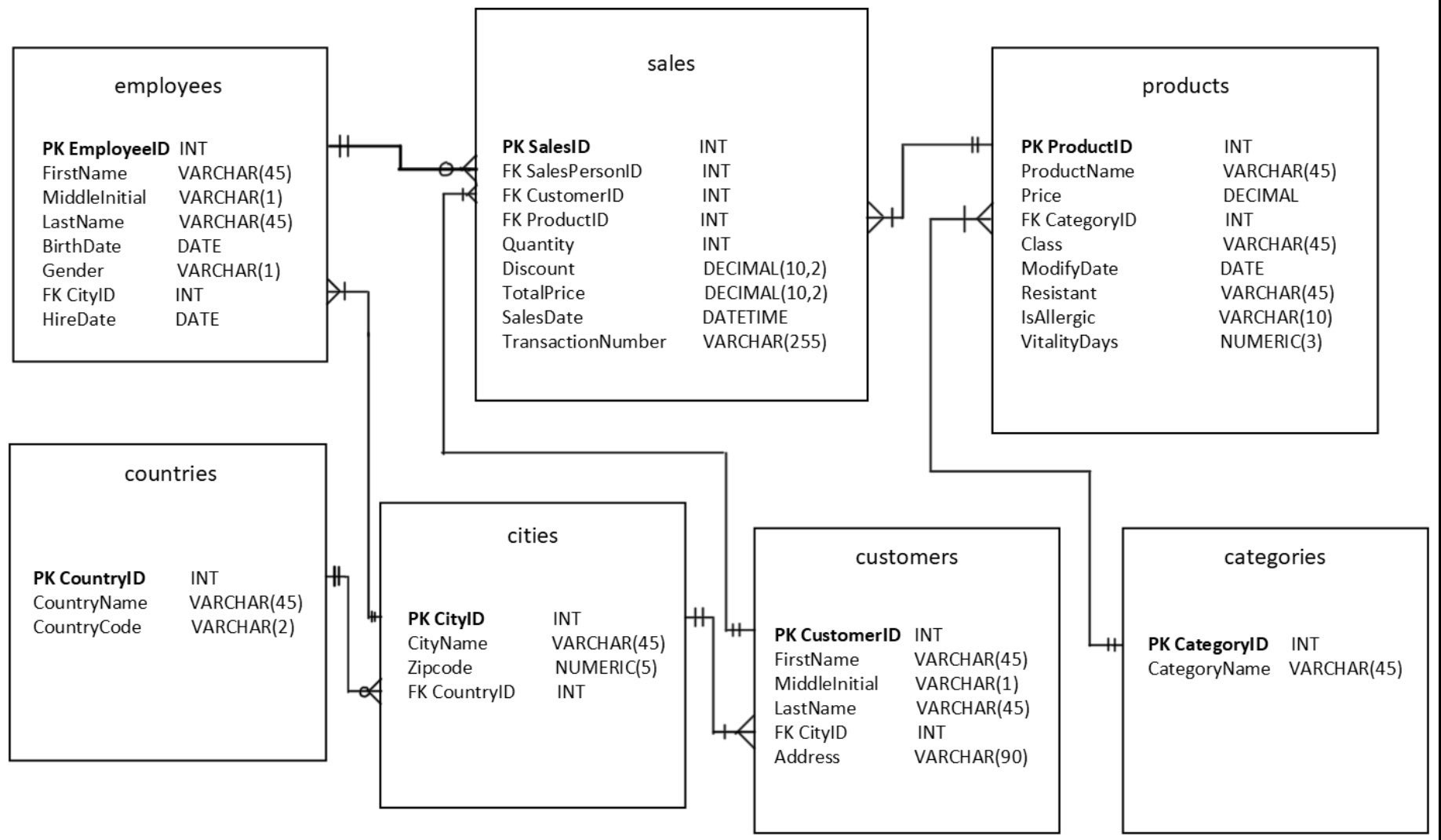
Relationships Between Tables

1. Foreign Key Relationships

Each ProductID in the sales table is a foreign key that references the primary key in the products table. This is a one-to-many relationship, where one product can have many sales records.

Each CustomerID in the sales table is a foreign key that references the primary key in the customers table. This also constitutes a one-to-many relationship, where one customer can have many sales records.

Each CityID in the customers table is a foreign key that references the primary key in the cities table, and each CountryID in the cities table is a foreign key that references the primary key in the countries table. Both are one-to-many relationships, where one city can have many customers, and one country can have many cities.

Each CategoryID in the products table is a foreign key that references the primary key in the categories table. This is a one-to-many relationship, as one category can include many products.

Each SalesPersonID in the sales table is a foreign key that references the primary key in the employees table. This is a one-to-many relationship, where one salesperson can be associated with many sales transactions.

2. Referential Integrity Constraints

These constraints ensure that the foreign key fields must match the primary key that is referenced in another table or must be null. This maintains the consistency and integrity of the data across the tables.

3. Normalization

The database design suggests that it is normalized, which means the data is organized into tables in such a way that redundancy is minimized. For example, customer information is stored in a separate customers table and not repeated in the sales table.

Part 2: Database Schema

Part 3 – Schema and Database Creation Script

Schema and Database Creation Script

CREATE SCHEMA IF NOT EXISTS termproject;
USE termproject;
-- Create the sales table if it doesn't exist
CREATE TABLE IF NOT EXISTS sales (
    	SalesID INT PRIMARY KEY,
    	SalesPersonID INT,
   	CustomerID INT,
   	ProductID INT,
   	Quantity INT,
    	Discount NUMERIC,
  	TotalPrice DECIMAL(10,2),
  	SalesDate DATETIME, /*fixed*/
  	TransactionNumber VARCHAR(255));
CREATE TABLE IF NOT EXISTS categories (
	CategoryID INT PRIMARY KEY,
CategoryName VARCHAR(45));
CREATE TABLE IF NOT EXISTS cities(
	CityID INT PRIMARY KEY,
CityName VARCHAR(45),
Zipcode NUMERIC(5),
    	CountryID INTEGER REFERENCES countries (CountryID) ON DELETE RESTRICT);
CREATE TABLE IF NOT EXISTS countries(
	CountryID INT PRIMARY KEY,
    	CountryName VARCHAR(45),
   	CountryCode VARCHAR(2));
CREATE TABLE IF NOT EXISTS customers(
	CustomerID INT PRIMARY KEY,
    	FirstName VARCHAR(45),
   	MiddleInitial VARCHAR(1),
    	LastName VARCHAR(45),
    	CityID INT REFERENCES cities (CityID) ON DELETE RESTRICT,
    	Address VARCHAR(90));
CREATE TABLE IF NOT EXISTS employees(
	EmployeeID INT PRIMARY KEY,
    	FirstName VARCHAR(45),
MiddleInitial VARCHAR(1),
LastName VARCHAR(45),
BirthDate DATE,
Gender VARCHAR(1),
CityID INT REFERENCES Cities (CityID) ON DELETE RESTRICT,
HireDate DATE);
CREATE TABLE IF NOT EXISTS products(
ProductID INT PRIMARY KEY,
ProductName VARCHAR(45),
Price DECIMAL,
CategoryID INT REFERENCES categories (CategoryID) ON DELETE RESTRICT,  -- Fixed case
Class VARCHAR(45),
ModifyDate DATE,
Resistant VARCHAR(45),
IsAllergic VARCHAR(10) CHECK (IsAllergic IN ('True','False','Unknown')),  -- More flexible
VitalityDays NUMERIC(3));

Part 4: SQL Queries and Analysis

Data Import Complications

In the journey of transforming raw data into meaningful insights, the initial step of importing data into a database often poses unforeseen challenges. This was certainly the case in our grocery data analysis project, where the process of transferring data from various CSV files into a MySQL database presented a series of complications that necessitated meticulous troubleshooting and adaptation. These issues ranged from incompatible file formats and encoding discrepancies to data integrity concerns and hardware limitations.

Such challenges underscore the importance of flexibility and problem-solving in data analysis, where the seemingly straightforward task of data import can quickly evolve into a complex endeavor requiring a deep understanding of both the data and the tools at hand. This section delves into the specific obstacles encountered during the data import process, providing a detailed account of the strategies employed to overcome them and the lessons learned in navigating the intricacies of data preparation.

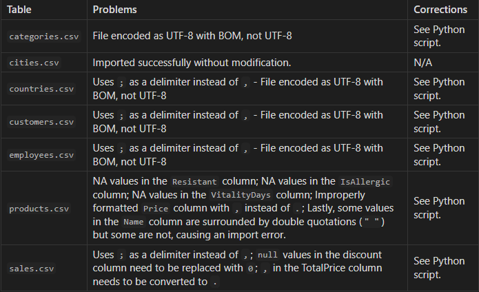
Fixing `categories.csv` for import

This file uses ; as a delimiter instead of , which inhibits import in both MySQL and Google BigQuery.

Uses UTF-8 with BOM, not clean UTF-8 encoding.

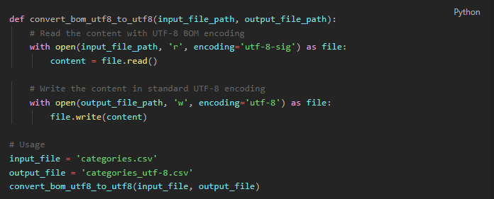
Fixing `countries.csv` for import

This file uses ; as a delimiter instead of , which inhibits import in both MySQL and Google BigQuery.

Uses UTF-8 with BOM, not clean UTF-8 encoding.

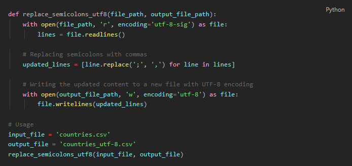
Fixing `customers.csv` for import

This file uses ; as a delimiter instead of , which inhibits import in both MySQL and Google BigQuery.

Uses UTF-8 with BOM, not clean UTF-8 encoding.

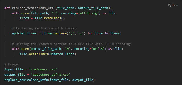
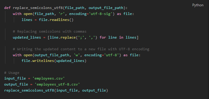
Fixing `employees.csv` for import

This file uses ; as a delimiter instead of , which inhibits import in both MySQL and Google BigQuery.

Uses UTF-8 with BOM, not clean UTF-8 encoding.

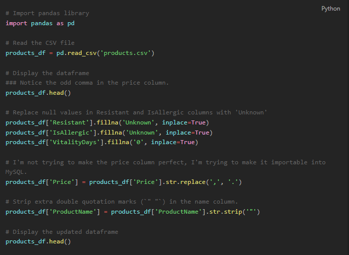
Fixing `products.csv` for import

Importing the original file failed due to:

NA values in the Resistant column

NA values in the IsAllergic column

NA values in the VitalityDays column

Improperly formatted Price column with , instead of ..

Lastly, some values in the Name column are surrounded by double quotations (" ") but some are not, causing an import error.

The following code takes products.csv as its input and returns products-cleaned.csv.

Fixing `sales.csv` for import

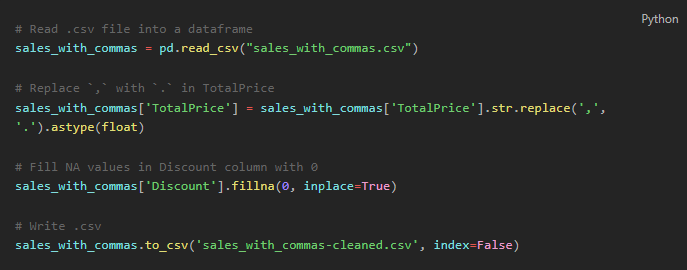
Uses ; as a delimiter instead of ,;

null values in the discount column need to be replaced with 0;

, in the TotalPrice column needs to be converted to .

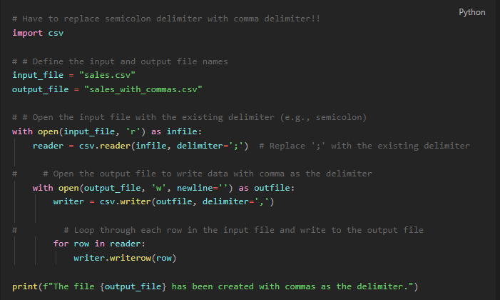
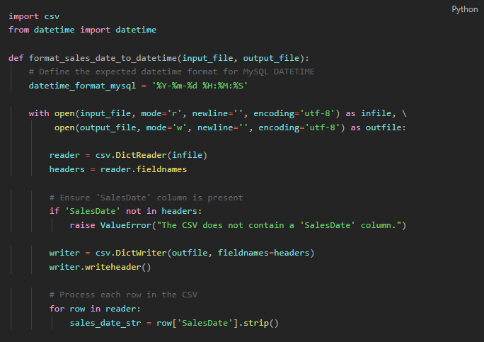
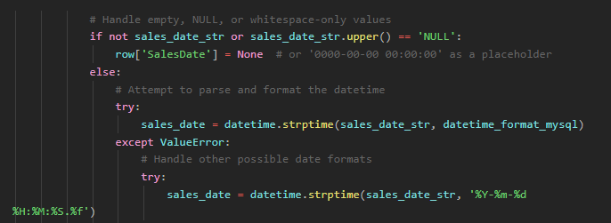
Lastly, DateTime formatting errors are preventing import.

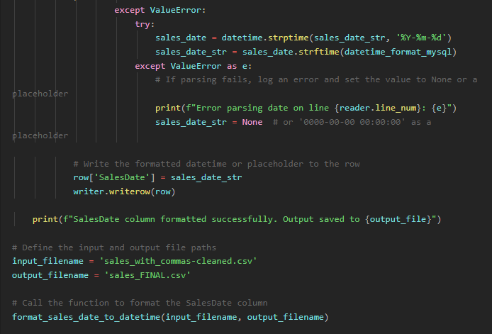
I abandoned efforts to import these data into MySQL. My PC does not have the processing power to execute this operation locally. Instead, I uploaded the files to my Google Cloud storage cluster and began SQL queries via Google BigQuery.

6.6 million lines is too much for one PC. This calls for cloud computing.

Fixing Product Prices in Sales Table in SQL

After importing all 6.6 million lines of sales.csv into BigQuery and beginning EDA, I found that all of the values for TotalPrice were empty. To resolve this issue, I joined the prices from the Products table onto the sales table and set TotalPrice equal to quantity multiplied by the updated price.

Exploratory Data Analysis

Unique Countries

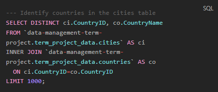
The SQL query is designed to extract distinct records that identify countries from the cities table and join them with the CountryName from the countries table. The use of INNER JOIN suggests that the query will only return the matching records where there is a correspondence between CountryID in both cities and countries tables.

From the screenshot of the query result, we observe that despite the countries table containing 206 distinct entries, indicative of a broad international dataset, the actual outcome reveals a narrower scope. The result set includes only one country, the United States, implying that the cities within the cities table are exclusively from this country. This limits the geographical breadth of any analysis to be conducted solely within the context of the United States.

In summary, while the countries table suggests a dataset with global coverage, the actual sales data from the cities table is geographically constrained to the United States. This result significantly narrows the analytical scope to U.S. cities only, thus shaping any subsequent data exploration or business insights to be region-specific.

Time Scope of Data

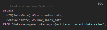
This query performs two aggregate functions on the SalesDate column of the sales table:

MIN(SalesDate) AS min_sales_date: This function finds the earliest (minimum) date in the SalesDate column, labeling the result as min_sales_date.

MAX(SalesDate) AS max_sales_date: This function finds the latest (maximum) date in the SalesDate column, labeling the result as max_sales_date.

The results from the query show that the earliest sales date (min_sales_date) is January 1, 2018, and the latest sales date (max_sales_date) is May 9, 2018. This indicates that the data within the sales table covers a period from the start of 2018 to just over the first week of May in the same year.

From this output, we can conclude that the dataset encompasses a little over four months of sales data, limiting any analysis to the first quarter (Q1) and part of the second quarter (Q2) of 2018. Due to this limited timeframe, it would indeed be insufficient to conduct analyses that require a longer temporal scope, such as seasonality trends, year-over-year growth, or quarter-over-quarter comparisons. Such analyses typically require at least one full year of data to account for seasonal variations and other temporal trends that could influence sales data. The restricted time span in this dataset precludes those kinds of temporal analyses and indicates that any conclusions drawn would be constrained to the early part of 2018 only.

Prices

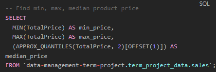
This query calculates three different statistics:

MIN(TotalPrice) AS min_price: This function finds the lowest price in the TotalPrice column, labeling the result as min_price.

MAX(TotalPrice) AS max_price: This function finds the highest price in the TotalPrice column, labeling the result as max_price.

(APPROX_QUANTILES(TotalPrice, 2)[OFFSET(1)]) AS median_price: This part of the query calculates the median of the TotalPrice column. Since the median is the middle value in a list of numbers, this function approximates the median by dividing the dataset into two quantiles (the parameter 2 in the function indicates the number of quantiles) and then picking the first element from the second quantile, which corresponds to the median.

The results indicate that the range of product prices in the sales table varies widely:

The min_price is $0.04, suggesting that the cheapest product sold is very low in cost.

The max_price is $2496.89, indicating a significant premium product or order within the dataset.

The median_price is $486.13, which provides a more robust measure of central tendency than the average would because it is less affected by the wide range of prices and the presence of extremely high or low values.

These figures help to understand the pricing behavior of the products sold. The large difference between the minimum and maximum prices may suggest a wide variety of products or services being sold, from very inexpensive to high-end items. The median price being closer to the maximum price than the minimum indicates that at least half of the products are priced above $486.13, which might suggest that the data skews towards more expensive items or that there are some high-value transactions elevating the median. Without additional context, such as the types of products sold or the volume of sales at each price point, it's challenging to draw definitive conclusions from these numbers alone. However, they do provide a snapshot of the pricing structure within the sales data.

Sales Insights

What is the total revenue by quarter/year?

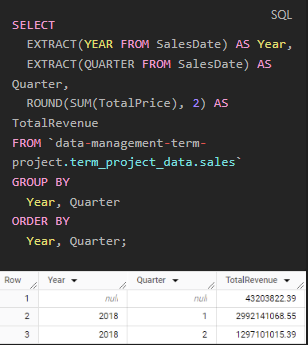
The SQL query below is designed to calculate the total revenue by year and quarter from the sales table. Here's how the query works:

EXTRACT(YEAR FROM SalesDate) AS Year: This function extracts the year component from the SalesDate column and labels it as Year.

EXTRACT(QUARTER FROM SalesDate) AS Quarter: This function extracts the quarter component from the SalesDate column, with quarters ranging from 1 to 4, and labels it as Quarter.

ROUND(SUM(TotalPrice), 2) AS TotalRevenue: This part of the query sums up the TotalPrice of all sales for each group (year and quarter) and rounds the result to two decimal places, labeling it as TotalRevenue.

GROUP BY Year, Quarter: This clause groups the results by the year and quarter, so that the revenue is calculated separately for each time period.

ORDER BY Year, Quarter: This sorts the results by year and quarter in ascending order.

The null values for Year and Quarter in the first row with a total revenue of $43,028,322.39 suggest that there are sales entries in the database without a specified sales date, as such entries would not have a year or quarter to extract. This amount is most likely an aggregation of all the sales records where the SalesDate is missing or null.

The second row shows the total revenue for the first quarter of 2018 (Q1), which amounts to $29,921,410.85. This quarter would encompass January, February, and March.

The third row represents the total revenue for the second quarter of 2018 (Q2), which is $12,971,010.15. However, because the dataset only goes up to May 9, 2018, this figure only includes sales from April 1, 2018, to May 9, 2018, and does not represent the entire second quarter.

This partial data for Q2 means that any analysis of that quarter would be incomplete, as it lacks nearly two months of potential sales data. Consequently, the reported revenue for Q2 cannot be directly compared to Q1 or used to extrapolate full-quarter performance. Moreover, the incomplete nature of the dataset precludes any meaningful analysis of trends beyond the scope of the available data. Any interpretation of sales performance, patterns, or trends would need to take this data limitation into account.

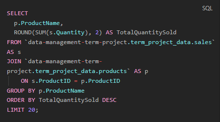
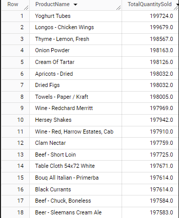
Which 20 products have the highest sales volume?

The result indicates that the product with the highest sales volume in the provided data is "Yogurt Tubes," with a total quantity sold of 199724.0 units. This information is derived from the SQL query which calculates the sum of quantities sold for each product, groups the results by product name, and orders them in descending order to list the top 20 products with the highest sales volume.

The query is well-structured for providing a clear and direct answer to which products have the highest volume of sales. By limiting the results to the top 20, it allows for a focused look at the best-performing products in terms of quantity sold. This kind of analysis is valuable for inventory management, marketing strategies, and understanding consumer demand within the dataset's time frame.

What is the average discount applied to sales transactions?

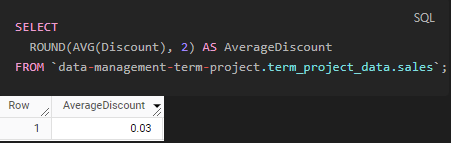
The SQL query calculates the average discount applied to sales transactions in the sales table of the project database and rounds this average to two decimal places. The result, as shown in the screenshot, indicates that the average discount is 0.03, or 3%.

From a business perspective, the average discount of 3% on sales transactions, as shown by the SQL query result, suggests a conservative discounting strategy. This indicates a focus on profitability and maintaining the perceived value of products rather than driving sales through significant price reductions. This metric is valuable for evaluating the effectiveness of the company's pricing strategy, marketing promotions, and for financial forecasting. It's also a useful benchmark for comparing the company's pricing policies against industry norms or competitors' practices.

How does the discount level affect the total sales volume?

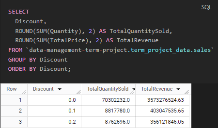
The SQL query calculates the total quantity sold and the total revenue generated for each level of discount applied to sales transactions. It groups the sales data by the discount percentage and sorts the results in ascending order of discounts. The query performs the following operations:

SELECT Discount: This selects the distinct discount values from the sales data.

ROUND(SUM(Quantity), 2) AS TotalQuantitySold: For each discount level, it calculates the total quantity of products sold and rounds this number to two decimal places.

ROUND(SUM(TotalPrice), 2) AS TotalRevenue: It also calculates the total revenue for each discount level and rounds this number to two decimal places.

FROM data-management-term-project.term_project_data.sales: This specifies the sales table from which to retrieve the data.

GROUP BY Discount: This groups the data by the discount percentage so that all sales with the same discount are aggregated together.

ORDER BY Discount: This orders the results by the discount percentage in ascending order.

The output of the query shows:

At a 0% discount, a total of 7,030,223.0 units were sold, resulting in revenue of $357,372,524.63.

A 10% discount saw a higher quantity sold at 8,817,780.0 units and increased revenue of $430,047,535.65.

A 20% discount resulted in a slightly lower quantity sold at 8,762,596.0 units compared to the 10% discount, and a reduced total revenue of $356,121,846.05.

This data suggests that a moderate 10% discount is optimal for increasing both sales volume and revenue, whereas a higher discount of 20% does not seem to stimulate additional sales volume to offset the lower prices, thus reducing overall revenue.

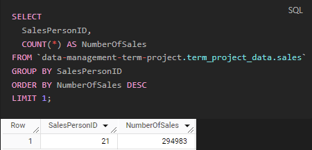
Which salesperson has the highest number of sales?

This SQL query identifies the salesperson with the highest number of sales by counting the number of sales transactions associated with each SalesPersonID. The steps of the query are as follows:

SELECT SalesPersonID: This selects the unique identifier for each salesperson.

COUNT(*) AS NumberOfSales: This counts the total number of sales transactions for each salesperson.

FROM data-management-term-project.term_project_data.sales: This specifies the sales table as the data source.

GROUP BY SalesPersonID: This groups the results by salesperson, which is necessary for the COUNT function to calculate the number of sales per salesperson.

ORDER BY NumberOfSales DESC: This orders the results in descending order by the number of sales, so the salesperson with the most sales is at the top.

LIMIT 1: This limits the results to only the top record, which shows the salesperson with the highest number of sales.

According to the query result in the screenshot, the salesperson with SalesPersonID 21 has the highest number of sales, totaling 29,483 transactions. By manually consulting the employees table, it is found that the salesperson's name is Devon Brewer. Therefore, Devon Brewer is the top-performing salesperson in terms of the number of sales transactions.

Product Performance

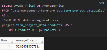
What is the average price of products sold?

This SQL query calculates the average price of products sold by joining the sales and products tables on the ProductID and then averaging the Price column from the products table. The result of this query, as shown in the screenshot, indicates that the average price of products sold is approximately $50.82. This figure helps in understanding the typical price point of products that the business sells, which can inform pricing strategies, marketing campaigns, and inventory decisions.

Are there products that stand out in terms of sales or lack thereof?

Highest Sales Volume

The SQL query provided retrieves information about the products with the highest sales volumes by summing the quantity sold for each product and ordering the results in descending order. The query results in a list of the top 10 products with the highest total quantities sold.

"Yogurt Tubes" have the highest total quantity sold, making it the standout product in terms of sales volume.

"Longos - Chicken Wings" and "Thyme - Lemon, Fresh" follow closely behind.

Other products like "Onion Powder," "Cream Of Tartar," and various others make up the remainder of the top 10 list.

These products are evidently the top performers in this dataset, indicating strong consumer demand or successful sales strategies for these items. They could be considered as key products for the business, potentially contributing a significant portion of sales revenue. The presence of these products at the top of the sales volume list suggests that they are likely to be crucial to inventory planning, marketing focus, and sales forecasting.

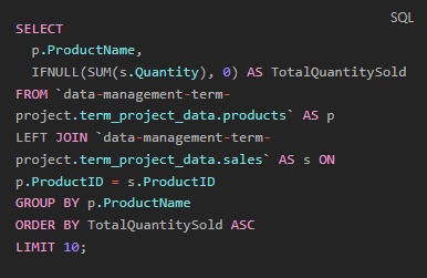
Lowest Sales Volume

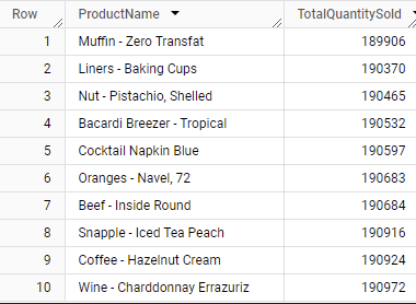
This SQL query retrieves information about the products with the lowest sales volumes by summing the quantity sold for each product, accounting for the possibility of null values with the IFNULL function. The results are ordered in ascending order to show the products with the least quantity sold.

"Muffin - Zero Transfat" appears to have the lowest total quantity sold among the products listed, suggesting it may not be as popular or in demand as other items.

Products such as "Liners - Baking Cups," "Nut - Pistachio, Shelled," and "Bacardi Breezer - Tropical" are also on the lower end of the sales volume spectrum.

The list includes a mix of items from different categories, indicating a varied range of products that are not selling as well as others.

These products might be underperforming in sales compared to others in the inventory, which could be due to several factors such as consumer preference, pricing, competition, or lack of promotion. Businesses could use this data to investigate the reasons behind the low sales volume and consider strategies such as marketing initiatives, price adjustments, or even discontinuing the products to optimize sales and inventory management.

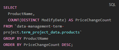
How often do product prices change (based on `ModifyDate`)?

This SQL query is designed to count the number of unique modification dates for each product, which serves as a proxy for the frequency of price changes. Here’s how it works:

It selects the ProductName.

It counts the distinct ModifyDate entries for each product, which is represented by PriceChangeCount. A distinct count here is used to ensure that if the price was modified multiple times on the same date, it would only be counted once.

The data is then grouped by ProductName to ensure the count is specific to each product.

Finally, it orders the results by PriceChangeCount in descending order, so the products with the most price changes are listed first.

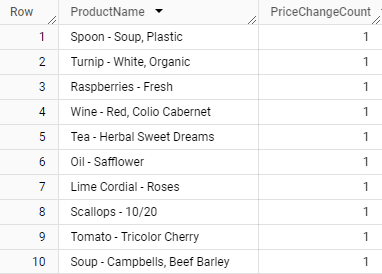
The result shows that for the top 10 products listed, each has a PriceChangeCount of 1. This indicates that across the dataset, each of these products has had its price changed only once. This might suggest a relatively stable pricing strategy for these products or that the dataset does not cover a long enough time period to reflect multiple price changes. If prices are not changed frequently, this could mean that the business does not often use price adjustments as a competitive strategy or response to market dynamics, or it could reflect a period of stable supply costs and market demand.

Customer Analysis

Who are the top 10 customers by sales volume?

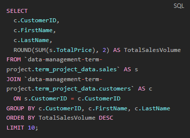
The SQL query below compiles a list of the top 10 customers based on their total sales volume. It joins the sales and customers tables on the CustomerID to associate sales with the correct customer and sums the TotalPrice of sales for each customer. It then rounds this sum to two decimal places and groups the results by CustomerID, FirstName, and LastName to ensure each customer is uniquely identified. The customers are ordered by their TotalSalesVolume in descending order, showing those with the highest sales volume at the top of the list.

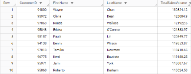
The query returns a list of the top 10 customers with their CustomerID, FirstName, LastName, and their corresponding TotalSalesVolume. The customer at the top of the list, with the highest total sales volume, is Wayne Chan, followed by other customers with slightly lower sales volumes. These top customers are likely to be of particular importance to the business due to their high sales volume, potentially qualifying for VIP treatment, targeted marketing campaigns, or loyalty programs. Understanding who the top customers are can help the business tailor its customer relationship management strategies effectively.

What are the purchasing patterns of customers from different cities in the United States?

Purchasing Frequency: Top 20 city markets by purchase frequency

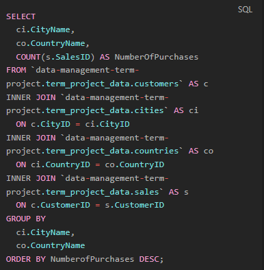
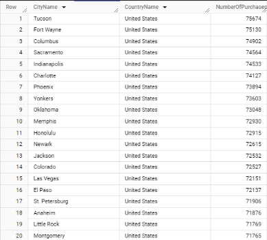
This SQL query analyzes the purchasing patterns of customers from different cities in the United States by counting the number of purchases made in each city. It does this by joining the customers, cities, countries, and sales tables on their respective IDs. After aggregating the sales by city and country, it groups the results by CityName and CountryName to ensure the purchase frequency is associated with the correct location. The results are then ordered by the number of purchases in descending order, showcasing the cities with the most active buying behavior at the top.

The data reveals the top 20 U.S. city markets by purchase frequency. The city with the highest number of purchases is Tucson, followed by Fort Wayne, Columbus, and others down the list. This information indicates which city markets are the most active in terms of purchase frequency and could guide targeted marketing strategies, inventory distribution, and expansion planning. Cities with higher purchasing frequencies might suggest a stronger market presence or customer base, warranting more focused attention from sales and marketing efforts.

Average Sale Amount: Top 20 markets by average sale amount

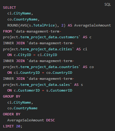
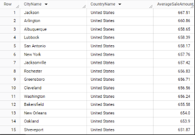
This SQL query calculates the average sale amount per city by joining customer, city, country, and sales tables, and then averaging the total price of sales for each city. The results are grouped by CityName and CountryName and ordered by the average sale amount in descending order to identify the top 20 markets with the highest average transaction value.

In the result, we see the top 15 U.S. markets by average sale amount. For an undetermined reason, only 15 lines displayed with a LIMIT 20, likely due to null values. Jackson leads with the highest average sale amount, followed by Arlington, Albuquerque, and others on the list. These figures indicate the average revenue per sale transaction in each city, which can be a useful indicator of customer spending behavior in different locations.

For a business, understanding the markets where customers spend more per transaction can inform strategic decisions such as where to allocate marketing resources, where to focus customer service efforts, or where to stock higher-value inventory. Additionally, it could also suggest areas with higher disposable income or a preference for premium products, guiding product mix and promotional strategies.

Most Popular Products

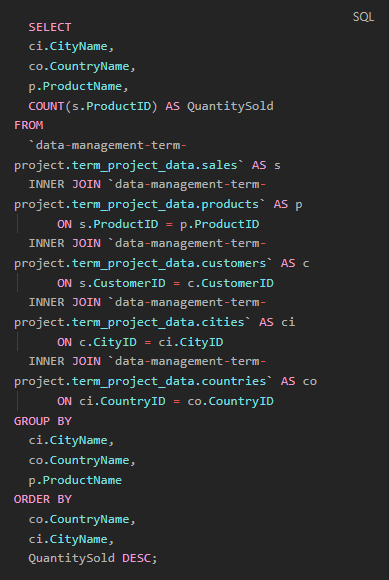
This SQL query is structured to identify the most popular products among customers in each city within the United States. It does this by:

Joining the sales, products, customers, cities, and countries tables to consolidate sales data with product and customer location information.

Counting the number of times each product has been sold (COUNT(s.ProductID)), which is labeled as QuantitySold.

Grouping the results by CityName, CountryName, and ProductName to ensure the counts are specific to each product within each city.

Ordering the results first by CountryName and CityName to organize the data by location, and then by QuantitySold in descending order to rank the products within each city by popularity.

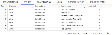
This query provides valuable insights into local consumer preferences, which can inform inventory decisions, marketing campaigns, and product development. By understanding which products are most popular in specific locations, a business can tailor its approach to meet the demands of each market effectively. This localized strategy could potentially lead to increased customer satisfaction and sales performance.

Seasonal Trends

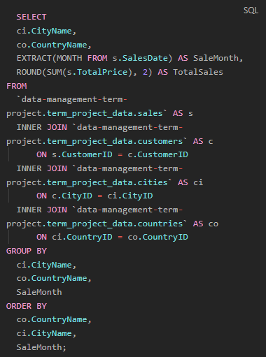
The SQL query is intended to uncover seasonal trends in purchasing patterns by city or country by extracting the month from the sales date and summing the total sales for each month. The results are then grouped by city, country, and sale month to see the variations in sales over different months.

However, the usefulness of this query for identifying seasonal trends is limited due to the dataset's timeframe, which only spans from January 1, 2018, to May 9, 2018. Seasonality analysis typically requires a full year of data, or even multiple years, to capture variations across all seasons and to account for events such as holidays, weather changes, and other seasonal factors that can significantly affect purchasing behavior.

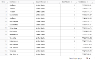
With only data from the first five months of the year, the analysis would not cover summer, fall, and early winter sales trends, including major holiday periods which could be critical for certain products or regions. Consequently, the results from this truncated dataset would not provide a comprehensive view of seasonal trends.

The results shown in the screenshot reflect this limitation, with data only available for a subset of the year. Without a complete annual cycle, it's impossible to identify patterns such as increased sales in specific months due to holidays or seasonal changes, making any conclusions about seasonality speculative at best. For accurate seasonal trend analysis, the dataset would need to encompass sales data from the entire year and preferably multiple years to account for year-over-year variability.

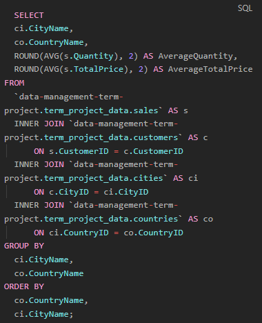
Purchase Size

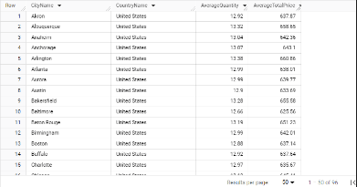
This SQL query examines the size of purchases by customers from each city, using the average quantity of items purchased and the average total price of those purchases as indicators. It does so by averaging the Quantity and TotalPrice of sales for each city after joining the relevant tables. The results are then grouped by CityName and CountryName to ensure they are specific to each location.

The output lists cities in the United States with the corresponding average quantity of items purchased and the average total price of purchases. The results can be used to compare purchasing behaviors across different cities.

Understanding the average purchase size in terms of quantity and total price can help businesses tailor their inventory, marketing, and pricing strategies to suit the preferences and spending habits of customers in specific locations. For instance, cities with higher average purchase sizes might be targeted for bulk sales promotions, whereas cities with lower average purchase sizes could be more receptive to marketing strategies that encourage larger basket sizes. This data can also assist in forecasting demand, optimizing stock levels, and planning logistics and distribution.

Distinct Customer Segments

This SQL query is designed to segment customers based on their purchasing behavior. It uses various metrics such as purchase frequency, total money spent, average purchase value, and the date of the last purchase to categorize customers. The segmentation is done using CASE statements to classify customers into spending categories ('High Spender', 'Medium Spender', 'Low Spender') based on their total spend, and frequency categories ('Frequent Buyer', 'Occasional Buyer', 'Infrequent Buyer') based on their purchase frequency.Here's a summary of how each part of the query contributes to customer segmentation:

COUNT(s.SalesID) counts the number of sales per customer, indicating how often they purchase.

ROUND(SUM(s.TotalPrice),2) calculates the total amount spent by each customer.

ROUND(AVG(s.TotalPrice), 2) finds the average value of a customer's purchase.

MAX(s.SalesDate) identifies the most recent purchase date for each customer.

The first CASE statement classifies customers into spending categories based on the total amount spent.

The second CASE statement classifies customers into frequency categories based on how many purchases they've made.

The results of this query allow a business to identify different customer segments such as 'High Spender - Frequent Buyer' or 'Low Spender - Infrequent Buyer'. This information is critical for targeted marketing, personalized customer service, and strategic sales planning. For instance, 'High Spender - Frequent Buyer' customers could be targeted with loyalty programs and exclusive offers, while 'Low Spender - Infrequent Buyer' customers might be encouraged with discounts or product recommendations to increase their purchase frequency and spending.

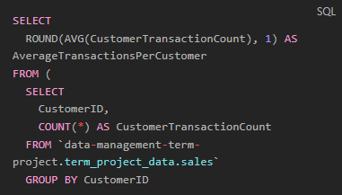
Average Transactions Per Customer

The SQL query calculates the average number of transactions per customer by first counting the number of transactions for each customer and then averaging those counts. The inner query:

Selects CustomerID from the sales table,

Counts the number of transactions for each customer using COUNT(*) AS CustomerTransactionCount,

Groups the results by CustomerID to ensure the count is per customer.

The outer query then calculates the average of these transaction counts using AVG(CustomerTransactionCount) and rounds the result to one decimal place.

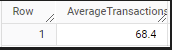
The result indicates that the average number of transactions per customer is 68.4. This metric provides insight into customer engagement, showing how frequently, on average, customers are making purchases. It can be a useful measure of customer loyalty and purchasing behavior for the business.

Summary of Findings

Our comprehensive analysis of grocery sales data, utilizing SQL queries complemented by Python preprocessing, has yielded several critical insights that paint a vivid picture of customer behaviors, sales dynamics, and product performance within the dataset.

Product Insights: 'Yogurt Tubes' emerged as a standout product, leading in sales volume. This finding indicates a significant market preference and points towards potential avenues for inventory focus and promotional strategies.

Customer Segmentation: Through intricate segmentation, customers were categorized into groups like 'High Spenders' and 'Frequent Buyers'. This segmentation is pivotal for developing targeted marketing campaigns and enhancing customer relationship management.

Geographic Trends: Analysis revealed key markets such as Tucson, Fort Wayne, and Columbus, exhibiting high purchase frequencies. These insights are instrumental for localized marketing strategies and inventory distribution decisions.

Transactional Analysis: The average transaction value varied significantly across cities, suggesting regional differences in spending patterns. This variation could inform differentiated marketing and inventory strategies to cater to regional preferences.

Data Quality and Management: Our project underscored the importance of robust data management practices. Initial challenges with data quality highlighted the need for regular data validation and cleaning protocols to ensure the integrity and reliability of future analyses.

Seasonal and Temporal Limitations: The dataset's coverage of the first five months of 2018 provided a constrained view of seasonal trends. For comprehensive seasonal analysis, a full year's data, or preferably multiple years, would be required.

Operational Insights: The analysis underscored the importance of efficient sales and inventory strategies, suggesting opportunities for optimization in these areas to enhance overall business performance.

In summary, our findings offer a multi-faceted understanding of the grocery data, enabling nuanced sales strategies and customer engagement approaches. These insights are not only crucial for addressing immediate business needs but also for paving the way for sustained growth and enhanced customer satisfaction in a competitive market.

Key Recommendations

The store owner should capitalize on the sales momentum of 'Yogurt Tubes' through focused cross-promotional strategies and consider bundling them with complementary items to increase the average purchase size. The segmentation analysis calls for a strategic focus on 'High Spender - Frequent Buyer' segments, which could be engaged through personalized marketing and exclusive loyalty initiatives. Regionally, the marketing efforts should be aligned with cities demonstrating higher purchase frequencies, employing tailored promotions to cater to these active markets. In cities with higher average transaction values, the introduction of premium products could leverage the purchasing power of these customers.

Crucially, the store must prioritize data quality management to ensure reliable data analysis. This entails establishing protocols for consistent data entry, regular data cleaning, and validation processes to prevent the import issues encountered, which required extensive corrections in Python before the data was usable for SQL queries. By improving data quality and leveraging the insights gained, the store can optimize its marketing and sales strategies to drive growth and enhance customer satisfaction.